
Digression Alert: Coding in R Blog

Years ago, I began a blog that was both a first-person narrative and a tutorial. If you don’t know, I am an adjunct professor who has used R to teach statistics and sports analytics. Sometimes I come across a problem that may not be necessary to teach to my students, but it’s still a learning opportunity, so I decided to share it in blog form.
Now that this Substack has its own life, I figured I would migrate those posts here. Hope this post helps you!
Learning Tidymodels with Baseball Data
Before the 2021 Major League Baseball season was completed, I attended my first L.A. R Users Group meeting where I was introduced to the tidymodels package. The name says it all: using syntax from the tidyverse to create statistical models. RStudio Software Engineer Max Kuhn walked us through how to create a number of statistical models, all in one straightforward workflow. The talk left me inspired both to master this package and to write this post.
I already code in the tidyverse because of how intuitive the language is and how easy it is to convey to others what I am trying to do. Communicating code and statistical approaches are paramount in my work. But I was inspired to write for another reason. Most educational lectures use datasets any statistical student has probably memorized. They are almost always useful in terms of understanding neat and tidy concepts and trends, but not always applicable to what a data scientist will actually study. So, as someone who’s made sports his vocation, I am always looking to find ways to adapt these tutorials to my domain. This post hopes to achieve teaching you a bit about tidymodels, baseball data and exposure to advanced modeling techniques in what could be the future of America’s Pastime.
Installing Necessary Packages
There are two main packages to install, the first is tidymodels itself:
install.packages("tidymodels")The second package will be for the data. While there are several resources to upload baseball data into your workspace, this tutorial will highlight the baseballrpackage.^[https://billpetti.github.io/baseballr/]. Bill Petti has done a masterful job keeping this package updated so that users can scrape the most sophisticated data from websites like Baseball-Reference.com. Note: this package can also scrape Baseball Savant and FanGraphs. To install this package:
# install.packages("devtools")
devtools::install_github("BillPetti/baseballr")
Exploring the Data
Runs scored and runs allowed have provided a clear foundation for explaining which teams win the most games. But which other factors should go into a model predicting the winning percentage for a team’s entire season?
This data acquisition is basically a three-step process: scrape team records, scrape team statistics from a separate location and join all into one dataframe. For this exercise I will only look at the last ten full seasons to where each row represents one team from one season (30 teams times 10 seasons = 300 observations). Using the standings_on_date_bref() command, here is how to scrape team standings:
al_standings_2011 <- standings_on_date_bref("2011-09-28", "AL Overall",
                                            from = FALSE)
nl_standings_2011 <- standings_on_date_bref("2011-09-28", "NL Overall",
                                            from = FALSE)
al_standings_2012 <- standings_on_date_bref("2012-10-03", "AL Overall",
                                            from = FALSE)
nl_standings_2012 <- standings_on_date_bref("2012-10-03", "NL Overall",
                                            from = FALSE)
al_standings_2013 <- standings_on_date_bref("2013-09-30", "AL Overall",
                                            from = FALSE)
nl_standings_2013 <- standings_on_date_bref("2013-09-30", "NL Overall",
                                            from = FALSE)
al_standings_2014 <- standings_on_date_bref("2014-09-28", "AL Overall",
                                            from = FALSE)
nl_standings_2014 <- standings_on_date_bref("2014-09-28", "NL Overall",
                                            from = FALSE)
al_standings_2015 <- standings_on_date_bref("2015-10-04", "AL Overall",
                                            from = FALSE)
nl_standings_2015 <- standings_on_date_bref("2015-10-04", "NL Overall",
                                            from = FALSE)
al_standings_2016 <- standings_on_date_bref("2016-10-02", "AL Overall",
                                            from = FALSE)
nl_standings_2016 <- standings_on_date_bref("2016-10-02", "NL Overall",
                                            from = FALSE)
al_standings_2017 <- standings_on_date_bref("2017-10-01", "AL Overall",
                                              from = FALSE)
nl_standings_2017 <- standings_on_date_bref("2017-10-01", "NL Overall",
                                              from = FALSE)
al_standings_2018 <- standings_on_date_bref("2018-10-01", "AL Overall",
                                            from = FALSE)
nl_standings_2018 <- standings_on_date_bref("2018-10-01", "NL Overall",
                                            from = FALSE)
al_standings_2019 <- standings_on_date_bref("2019-10-01", "AL Overall",
                                            from = FALSE)
nl_standings_2019 <- standings_on_date_bref("2019-10-01", "NL Overall",
                                            from = FALSE)
al_standings_2020 <- standings_on_date_bref("2020-09-27", "AL Overall",
                                            from = FALSE)
nl_standings_2020 <- standings_on_date_bref("2020-09-27", "NL Overall",
                                            from = FALSE)
standings_2011 <- dplyr::bind_rows(al_standings_2011$`AL Overall_up to_2011-09-28`,
                                   nl_standings_2011$`NL Overall_up to_2011-09-28`)
standings_2012 <- dplyr::bind_rows(al_standings_2012$`AL Overall_up to_2012-10-03`,
                                   nl_standings_2012$`NL Overall_up to_2012-10-03`)
standings_2013 <- dplyr::bind_rows(al_standings_2013$`AL Overall_up to_2013-09-30`,
                                   nl_standings_2013$`NL Overall_up to_2013-09-30`)
standings_2014 <- dplyr::bind_rows(al_standings_2014$`AL Overall_up to_2014-09-28`,
                                   nl_standings_2014$`NL Overall_up to_2014-09-28`)
standings_2015 <- dplyr::bind_rows(al_standings_2015$`AL Overall_up to_2015-10-04`,
                                   nl_standings_2015$`NL Overall_up to_2015-10-04`)
standings_2016 <- dplyr::bind_rows(al_standings_2016$`AL Overall_up to_2016-10-02`,
                                   nl_standings_2016$`NL Overall_up to_2016-10-02`)
standings_2017 <- dplyr::bind_rows(al_standings_2017$`AL Overall_up to_2017-10-01`,
                                   nl_standings_2017$`NL Overall_up to_2017-10-01`)
standings_2018 <- dplyr::bind_rows(al_standings_2018$`AL Overall_up to_2018-10-01`,
                                   nl_standings_2018$`NL Overall_up to_2018-10-01`)
standings_2019 <- dplyr::bind_rows(al_standings_2019$`AL Overall_up to_2019-10-01`,
                                   nl_standings_2019$`NL Overall_up to_2019-10-01`)
standings_2020 <- dplyr::bind_rows(al_standings_2020$`AL Overall_up to_2020-09-27`,
                                   nl_standings_2020$`NL Overall_up to_2020-09-27`)
While this command is straightforward, each season ended on different dates of the year, so I prefer creating a data frame writing redundant code to avoid missing games, as opposed to writing a “for loop”. A quick inspection of the first few results shows what’s assembled:
head(standings_2020)
# A tibble: 6 x 8
#  Tm        W     L `W-L%` GB       RS    RA `pythW-L%`
#  <chr> <int> <int>  <dbl> <chr> <int> <int>      <dbl>
#1 TBR      40    20  0.667 --      289   229      0.605
#2 MIN      36    24  0.6   4.0     269   215      0.601
#3 OAK      36    24  0.6   4.0     274   232      0.576
#4 CHW      35    25  0.583 5.0     306   246      0.599
#5 CLE      35    25  0.583 5.0     248   209      0.578
#6 NYY      33    27  0.55  7.0     315   270      0.57
Next, concerning explanatory variables, let’s look at standard batting box score statistics. I have performed similar exercises where I have combined hitting and pitching data, but often these dataframes cancel each other out, so for ease I will stick to just the offense. Here, statistics will be scraped more manually, so the XML and RCurl packages will be needed:
#install.packages("XML")
#install.packages("RCurl")
#https://cran.r-project.org/web/packages/XML/index.html and
#https://cran.r-project.org/web/packages/RCurl/index.html for more info
library(XML)
library(RCurl)

site_2020 <- paste0("https://www.baseball-reference.com/leagues/MLB/2020.shtml")
url_2020 <- getURL(site_2020)
batting_2020 <- readHTMLTable(url_2020)
batting_2020 <- batting_2020$teams_standard_batting %>% filter(Tm != 'LgAvg')

site_2019 <- paste0("https://www.baseball-reference.com/leagues/MLB/2019.shtml")
url_2019 <- getURL(site_2019)
batting_2019 <- readHTMLTable(url_2019)
batting_2019 <- batting_2019$teams_standard_batting %>% filter(Tm != 'LgAvg')

site_2018 <- paste0("https://www.baseball-reference.com/leagues/MLB/2018.shtml")
url_2018 <- getURL(site_2018)
batting_2018 <- readHTMLTable(url_2018)
batting_2018 <- batting_2018$teams_standard_batting %>% filter(Tm != 'LgAvg')

site_2017 <- paste0("https://www.baseball-reference.com/leagues/MLB/2017.shtml")
url_2017 <- getURL(site_2017)
batting_2017 <- readHTMLTable(url_2017)
batting_2017 <- batting_2017$teams_standard_batting %>% filter(Tm != 'LgAvg')

site_2016 <- paste0("https://www.baseball-reference.com/leagues/MLB/2016.shtml")
url_2016 <- getURL(site_2016)
batting_2016 <- readHTMLTable(url_2016)
batting_2016 <- batting_2016$teams_standard_batting %>% filter(Tm != 'LgAvg')

site_2015 <- paste0("https://www.baseball-reference.com/leagues/MLB/2015.shtml")
url_2015 <- getURL(site_2015)
batting_2015 <- readHTMLTable(url_2015)
batting_2015 <- batting_2015$teams_standard_batting %>% filter(Tm != 'LgAvg')

site_2014 <- paste0("https://www.baseball-reference.com/leagues/MLB/2014.shtml")
url_2014 <- getURL(site_2014)
batting_2014 <- readHTMLTable(url_2014)
batting_2014 <- batting_2014$teams_standard_batting %>% filter(Tm != 'LgAvg')

site_2013 <- paste0("https://www.baseball-reference.com/leagues/MLB/2013.shtml")
url_2013 <- getURL(site_2013)
batting_2013 <- readHTMLTable(url_2013)
batting_2013 <- batting_2013$teams_standard_batting %>% filter(Tm != 'LgAvg')

site_2012 <- paste0("https://www.baseball-reference.com/leagues/MLB/2012.shtml")
url_2012 <- getURL(site_2012)
batting_2012 <- readHTMLTable(url_2012)
batting_2012 <- batting_2012$teams_standard_batting %>% filter(Tm != 'LgAvg')

site_2011 <- paste0("https://www.baseball-reference.com/leagues/MLB/2011.shtml")
url_2011 <- getURL(site_2011)
batting_2011 <- readHTMLTable(url_2011)
batting_2011 <- batting_2011$teams_standard_batting %>% filter(Tm != 'LgAvg')
One thing to note is these batting tables include a league summary line that must be filtered out. Note: For a complete list of variable definitions, click here.
Again, one quick inspection of these data:
head(batting_2011)
#   Tm Bat BatAge  R/G   G   PA   AB   R    H  2B 3B  HR RBI  SB CS  BB   SO
#1 ARI   51   28.3 4.51 162 6096 5421 731 1357 293 37 172 702 133 55 531 1249
#2 ATL   45   28.9 3.96 162 6169 5528 641 1345 244 16 173 606  77 44 504 1260
#3 BAL   50   28.3 4.37 162 6156 5585 708 1434 273 13 191 684  81 25 452 1120
#4 BOS   49   30.0 5.40 162 6414 5710 875 1600 352 35 203 842 102 42 578 1108
#5 CHC   42   29.2 4.04 162 6130 5549 654 1423 285 36 148 610  69 23 425 1202
#6 CHW   42   30.0 4.04 162 6159 5502 654 1387 252 16 154 625  81 53 475  989
#    BA  OBP  SLG  OPS OPS+   TB GDP HBP SH SF IBB  LOB
#1 .250 .322 .413 .736   99 2240  82  61 50 33  55 1064
#2 .243 .308 .387 .695   90 2140 113  28 75 30  45 1109
#3 .257 .316 .413 .729   97 2306 154  52 24 43  24 1069
#4 .280 .349 .461 .810  116 2631 136  50 22 50  52 1190
#5 .256 .314 .401 .715   95 2224 123  59 60 35  35 1141
#6 .252 .319 .388 .706   89 2133 125  84 52 46  31 1126
Finally, it is time to merge each season’s batting and league standings dataframes, then join all 10 seasons together:
merge_2011 <- merge(batting_2011,standings_2011,by="Tm")
merge_2012 <- merge(batting_2012,standings_2012,by="Tm")
merge_2013 <- merge(batting_2013,standings_2013,by="Tm")
merge_2014 <- merge(batting_2014,standings_2014,by="Tm")
merge_2015 <- merge(batting_2015,standings_2015,by="Tm")
merge_2016 <- merge(batting_2016,standings_2016,by="Tm")
merge_2017 <- merge(batting_2017,standings_2017,by="Tm")
merge_2018 <- merge(batting_2018,standings_2018,by="Tm")
merge_2019 <- merge(batting_2019,standings_2019,by="Tm")
merge_2020 <- merge(batting_2020,standings_2020,by="Tm")

final_data <- rbind(merge_2011, merge_2012, merge_2013, merge_2014,
                    merge_2015, merge_2016, merge_2017, merge_2018,
                    merge_2019, merge_2020) %>% rename(record = 'W-L%')
One cosmetic change made was renaming W-L% to record since the previous name has characters that could cause coding problems in R. Now, one more quick inspection:
head(final_data)
#Tm #Bat BatAge  R/G   G   PA   AB   R    H  2B 3B  HR RBI  SB CS  BB   SO
#1 ARI   51   28.3 4.51 162 6096 5421 731 1357 293 37 172 702 133 55 531 1249
#2 ATL   45   28.9 3.96 162 6169 5528 641 1345 244 16 173 606  77 44 504 1260
#3 BAL   50   28.3 4.37 162 6156 5585 708 1434 273 13 191 684  81 25 452 1120
#4 BOS   49   30.0 5.40 162 6414 5710 875 1600 352 35 203 842 102 42 578 1108
#5 CHC   42   29.2 4.04 162 6130 5549 654 1423 285 36 148 610  69 23 425 1202
#6 CHW   42   30.0 4.04 162 6159 5502 654 1387 252 16 154 625  81 53 475  989
#    BA  OBP  SLG  OPS OPS+   TB GDP HBP SH SF IBB  LOB  W  L  record GB  RS
#1 .250 .322 .413 .736   99 2240  82  61 50 33  55 1064 94 68 0.580  8.0 731
#2 .243 .308 .387 .695   90 2140 113  28 75 30  45 1109 89 73 0.549 13.0 641
#3 .257 .316 .413 .729   97 2306 154  52 24 43  24 1069 69 93 0.426 28.0 708
#4 .280 .349 .461 .810  116 2631 136  50 22 50  52 1190 90 72 0.556  7.0 875
#5 .256 .314 .401 .715   95 2224 123  59 60 35  35 1141 71 91 0.438 31.0 654
#6 .252 .319 .388 .706   89 2133 125  84 52 46  31 1126 79 83 0.488 18.0 654
#   RA pythW-L%
#1 662    0.545
#2 605    0.526
#3 860    0.412
#4 737    0.578
#5 756    0.434
#6 706    0.465
This final dataframe features 300 observations: 30 teams and 10 seasons with basic hitting statistics merged with records, winning percentage, runs scored and runs allowed. However, there is one issue worth resolving at this stage: because of the way these data were scraped, what should be numeric variables are stored as characters:
sapply(final_data, class)
#        Tm        #Bat      BatAge         R/G           G          PA
"character" "character" "character" "character" "character" "character"
#         AB           R           H          2B          3B          HR
"character" "character" "character" "character" "character" "character"
#        RBI          SB          CS          BB          SO          BA
"character" "character" "character" "character" "character" "character"
#        OBP         SLG         OPS        OPS+          TB         GDP
"character" "character" "character" "character" "character" "character"
#        HBP          SH          SF         IBB         LOB           W
"character" "character" "character" "character" "character"   "integer"
#          L      record          GB          RS          RA    pythW-L%
#  "integer"   "numeric" "character"   "integer"   "integer"   "numeric"
Fortunately, there is a quick fix to change every variable except teams into a numeric. Changing classifications could be done in the first step of tidymodels, but often it is better to conduct some steps outside of the “pre-processing” stage if you want these changes to be permanent:
library(magrittr)
cols = c(2:36)
final_data[,cols] %<>% lapply(function(x) as.numeric(as.character(x)))
sapply(final_data, class)
#   Tm        #Bat      BatAge         R/G           G          PA
"character"   "numeric"   "numeric"   "numeric"   "numeric"   "numeric"
#         AB           R           H          2B          3B          HR
  "numeric"   "numeric"   "numeric"   "numeric"   "numeric"   "numeric"
#        RBI          SB          CS          BB          SO          BA
  "numeric"   "numeric"   "numeric"   "numeric"   "numeric"   "numeric"
#        OBP         SLG         OPS        OPS+          TB         GDP
  "numeric"   "numeric"   "numeric"   "numeric"   "numeric"   "numeric"
#        HBP          SH          SF         IBB         LOB           W
  "numeric"   "numeric"   "numeric"   "numeric"   "numeric"   "numeric"
#          L      record          GB          RS          RA    pythW-L%
  "numeric"   "numeric"   "numeric"   "numeric"   "numeric"   "numeric"
One issue that should be considered now involves which sets of variables to include. Because of COVID-19 concerns, Major League Baseball shortened its 2020 season. While every other season in the dataframe had 162 games, the 2020 campaign had only 60. Using variables signifying totals like total hits or total home runs would skew the results. Instead, explanatory variables representing averages should be normally distributed. While statistics like BA (batting average) are already in the dataframe, stolen bases, caught stealing and grounded into double play averages are not.
Let’s add those variables and also rename OPS+ so the “plus sign” doesn’t mess with any code:
final_data <- final_data %>%
  mutate(SB.avg = SB/G, CS.avg = CS/G, GDP.avg = GDP/G) %>%
  rename(OPS.plus = `OPS+`)
Now, we can proceed with tidymodels.
tidymodels
If you were to model a handful of these explanatory variables on win percentage to determine which modeling technique is most predictive, the process would be conventional:
run the models desired using training data
predict win percentage using testing data
choose the model that predicts the best using most important criteria for goodness-of-fit
Though tidymodels offers the same framework, the package has its own verbiage and workflow that, ultimately, will make model specification far easier and offer flexibility in tuning parameters necessary for more complex machine learning techniques.^[https://www.tidymodels.org/start/tuning/]
In the past, individual models would have to be coded individually. A linear regression would have its own block of code, a Bayesian model another block, etc., then it would be up to the user to save summary metrics to determine goodness-of-fit, not to mention dealing with each model having its own syntax. The caret package helped alleviate some of this burden by having a number of models available with ease. Consider tidymodels to be another evolutionary step in trying out a number of models with little effort. Other advantages to this package will become apparent at each step of the experiment.
Just like with any experiment, tidymodels can be broken down into three steps:
recipe
to preprocess data
to specify the models
prep
execute the models
bake
test models using testing data
A Simple Introduction
This dataframe–and the experiment–assumes uniformity, meaning it does not matter how the data are grouped between training and testing. Here, let’s perform an 80-20 split and set a seed so results are reproducible:
set.seed(1234)
data_split <- initial_split(final_data, prop = 0.80)
data_split

data_train <- training(data_split)
data_test  <-  testing(data_split)
Let’s first create a simple recipe to specify a linear regression:
simple_data <-
  recipe(record ~ OBP + SLG + OPS.plus + SB.avg
         + CS.avg + GDP.avg, data = data_train)
The astute data scientist and baseball fan might notice a problem. Components of OPS.plus already include OBP and SLG. There should be reasonable concerns for multi-collinearity. Fortunately, creating interaction terms is easy in tidymodels thanks to step functions. These commands allow for a variety of different pre-processing steps to occur to elements of the training data in just a few lines of code. Here’s how it is done with creating interaction terms using the step_interact() command:
simple_data <-
  recipe(record ~ OBP + SLG + OPS.plus + SB.avg
         + CS.avg + GDP.avg, data = data_train) %>%
  step_interact(recipe = simple_data, terms = ~ OBP:OPS.plus + SLG:OPS.plus) %>%
  prep()
simple_data
#Data Recipe

#Inputs:

#      role #variables
#   outcome          1
# predictor          6

#Training data contained 240 data points and no missing data.

#Operations:

#Interactions with OBP:OPS.plus + SLG:OPS.plus [trained]
The prepping stage was already included due to ease and the baking stage is straightforward with the one model:
test_ex <- bake(simple_data, new_data = data_test)
head(test_ex)
# A tibble: 6 x 9
#    OBP   SLG OPS.plus SB.avg CS.avg GDP.avg record OBP_x_OPS.plus
#  <dbl> <dbl>    <dbl>  <dbl>  <dbl>   <dbl>  <dbl>          <dbl>
#1 0.322 0.413       99  0.821  0.340   0.506  0.58            31.9
#2 0.308 0.387       90  0.475  0.272   0.698  0.549           27.7
#3 0.314 0.401       95  0.426  0.142   0.759  0.438           29.8
#4 0.325 0.425      102  0.580  0.191   0.704  0.593           33.2
#5 0.305 0.349       85  1.05   0.272   0.648  0.438           25.9
#6 0.292 0.348       84  0.772  0.247   0.506  0.414           24.5
# … with 1 more variable: OPS.plus_x_SLG <dbl>
The bake command creates a tibble of the test data with explanatory variables used (including interaction terms) and predictions for record.
If you want to look at the model itself, its summary metrics and predictions, a little backtracking is required. First, use the prep command again using the aforementioned recipe, but saved as a new object. One bit of advice Max Kuhn gave in his presentation was to use _fit in naming the model so the user is reminded it is a fitted model. Then, bake two things: one object using the training data and one with the testing. Next, create a model using the same variables but with the training data, use the glance() command to look at summary statistics, and then use the predict() command to see the results. The code looks like this with key output included:
data_rec_prepped <- prep(simple_data)
data_train_prepped <- bake(data_rec_prepped, new_data = NULL)
data_test_prepped <- bake(data_rec_prepped, data_test)

lm_fit <- lm(record ~ ., data = data_train_prepped)
glance(lm_fit)
# A tibble: 1 x 12
#  r.squared adj.r.squared  sigma statistic  p.value    df logLik   AIC   BIC
#      <dbl>         <dbl>  <dbl>     <dbl>    <dbl> <dbl>  <dbl> <dbl> #<dbl>
#1     0.472         0.454 0.0559      25.8 2.70e-28     8   356. -693. -658.

View(tidy(lm_fit))

predict(lm_fit, data_test_prepped %>% head())
#        1         2         3         4         5         6
#0.5123714 0.4431140 0.4952766 0.5352913 0.4599048 0.4092434
The View() command provides the following estimates and p-values for the model:
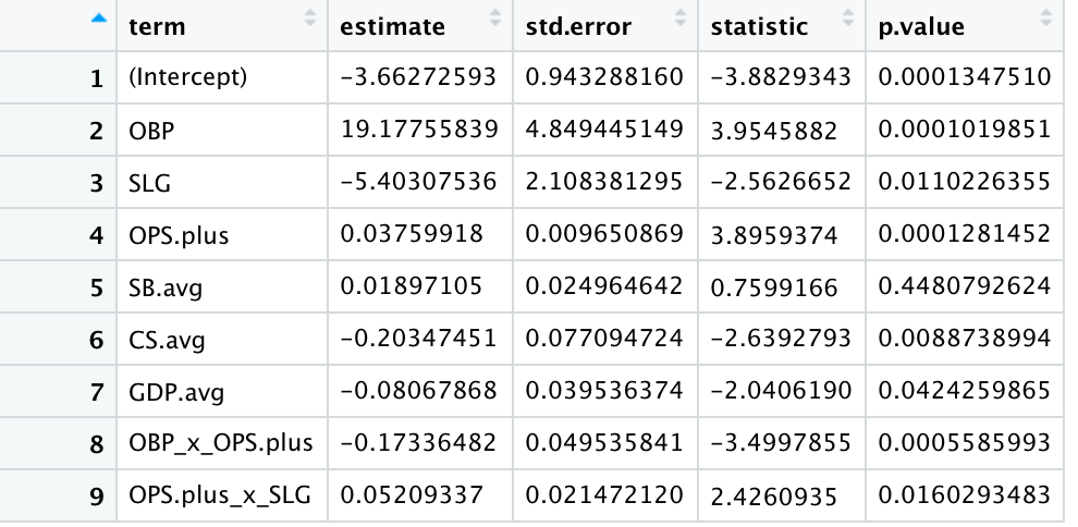
There is one coefficient that is not intuitive: SLG is a negative number where a predicted record goes down if slugging percentage goes up. However, the interaction term is positive. Also, the only variable with a p-value greater than .05 was stolen base average. Otherwise, every variable is statistically significant with 95% confidence.
The summary metrics show an r-squared of 0.472, which suggests some improvements should be made if any significant analysis were to be implemented. Again, pitching and defensive data would likely help goodness-of-fit, but for this tutorial, advanced modeling techniques could also be useful and will be the next approach.
A Workflow
Another advantage to tidymodels comes from the ability to streamline the model building and selection process, also called a workflow. The interface is simpler with fewer objects to keep track of, recipes and prep work are more easily executed and more advanced models can be summoned concisely.^[https://workflows.tidymodels.org]
Earlier, the simplified example used a basic linear model already included in R. More advanced models may need outside packages. Fortunately, the set_engine() command states which package or system is needed for the model that will be used. Think of the engine as setting the foundation where additional, more complex, models are based. For instance, as noted in the example, interaction terms were created for the linear model because of concerns about multi-collinearity. Principal Component Analysis (PCA) could also alleviate such concerns by reducing dimensionality to a smaller data set that is overall less correlated. Because PCA is an extension of a standard linear regression, the engine in our baseball experiment can be set to lm:
reg_model <- linear_reg() %>% set_engine("lm")Then, just like before, the user can create a recipe, only this time include the step_pca() and step_normalize() step functions to create a PCA and to center and scale numeric data, respectively. As a standard, let’s set the number of new features to 10:
pca_rec <- recipe(record ~ OBP + SLG + OPS.plus + SB.avg
                  + CS.avg + GDP.avg, data = data_train) %>%
  step_normalize(all_numeric_predictors()) %>%
  step_pca(all_numeric_predictors(), num_comp = 10)
A linear regression and a PCA model have been written. These models can now be part of one workflow:
pca_lm_wflow <- workflow() %>%
  add_model(reg_model) %>%
  add_recipe(pca_rec)
Using the fit() command, estimates can now be extracted from the training data and predictions from the testing data:
estimate <- fit(pca_lm_wflow, data_train)
predict(estimate, data_test)
# A tibble: 60 x 1
#   .pred
#   <dbl>
# 1 0.510
# 2 0.444
# 3 0.492
# 4 0.532
# 5 0.448
# 6 0.428
# 7 0.514
# 8 0.441
# 9 0.554
#10 0.637
# … with 50 more rows
Once again, the predict() command produces a tibble of predictions.
Ultimately this workflow is meant to determine which model best predicts. There are myriad of models to choose from. Previously, coding each and every model would be, to put it mildly, a pain. Even keeping track of appropriate options may not always be feasible, or is at the very least, time consuming. To streamline this process, the command parsnip::parsnip_addin() brings up not just available options for models, but the line will generate the code needed for the objects like the specification of tuning parameters, the engines, etc.:
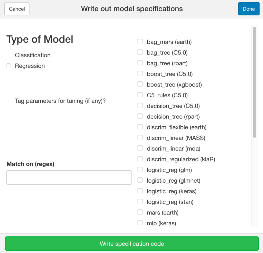
For this workflow, let’s utilize four different “approaches” to two models, a linear regression and a neural network. The latter can be specified this way:
nnet_model <-
  mlp(penalty = tune(), hidden_units = tune(), epochs = tune()) %>%
  set_engine("nnet") %>%
  set_mode("regression")
Next, let’s look at another PCA, except we “tune” the number of new features:
simple_rec <- recipe(record ~ OBP + SLG + OPS.plus + SB.avg
                     + CS.avg + GDP.avg, data = data_train) %>%
  step_normalize(all_numeric_predictors())

pca_rec <- simple_rec %>%
  step_pca(all_numeric_predictors(), num_comp = tune())
Two more categories are a partial least squares and a filtered approach with a high correlation filter:
pls_rec <- simple_rec %>%
  step_pls(all_numeric_predictors(), outcome = "record", num_comp = tune())

filter_rec <- simple_rec %>%
  step_corr(all_numeric_predictors(), threshold = tune())
All of these objects can now be included in a single workflow:
baseball_wflow <- workflow_set(
  preproc = list(basic = simple_rec, pca = pca_rec, pls = pls_rec,
                 filtered = filter_rec),
  models = list(lm = reg_model, nnet = nnet_model)
)
baseball_wflow
# A workflow set/tibble: 8 x 4
#  wflow_id      info             option      result
#  <chr>         <list>           <list>      <list>
#1 basic_lm      <tibble [1 × 4]> <wrkflw__ > <list [0]>
#2 basic_nnet    <tibble [1 × 4]> <wrkflw__ > <list [0]>
#3 pca_lm        <tibble [1 × 4]> <wrkflw__ > <list [0]>
#4 pca_nnet      <tibble [1 × 4]> <wrkflw__ > <list [0]>
#5 pls_lm        <tibble [1 × 4]> <wrkflw__ > <list [0]>
#6 pls_nnet      <tibble [1 × 4]> <wrkflw__ > <list [0]>
#7 filtered_lm   <tibble [1 × 4]> <wrkflw__ > <list [0]>
#8 filtered_nnet <tibble [1 × 4]> <wrkflw__ > <list [0]>
When this workflow is called up, all eight models are listed. But, if you look closely at the result column: nothing has been populated. All that has been done is state what the workflow is supposed to do, it has not been formally conducted.
To determine which model performs the best, we’ll use a bootstrapping approach with five partitions of the training data and one repeat of this V-fold partitioning. It is imperative to install the mixOmics first if it hasn’t been done already:
install.packages("BiocManager")
BiocManager::install('mixOmics')
As for the bootstrapping setup, setting a seed for reproducible results:
set.seed(999)
data_folds <- vfold_cv(data_train, v = 5, repeats = 1)
Now, it is time to execute the workflow using the workflow_map() command:
baseball_res <- baseball_wflow %>%
  workflow_map(resamples = data_folds,
               seed = 1,
               grid = 20)
baseball_res
# A workflow set/tibble: 8 x 4
#  wflow_id      info             option      result
#  <chr>         <list>           <list>      <list>
#1 basic_lm      <tibble [1 × 4]> <wrkflw__ > <rsmp[+]>
#2 basic_nnet    <tibble [1 × 4]> <wrkflw__ > <tune[+]>
#3 pca_lm        <tibble [1 × 4]> <wrkflw__ > <tune[+]>
#4 pca_nnet      <tibble [1 × 4]> <wrkflw__ > <tune[+]>
#5 pls_lm        <tibble [1 × 4]> <wrkflw__ > <tune[+]>
#6 pls_nnet      <tibble [1 × 4]> <wrkflw__ > <tune[+]>
#7 filtered_lm   <tibble [1 × 4]> <wrkflw__ > <tune[+]>
#8 filtered_nnet <tibble [1 × 4]> <wrkflw__ > <tune[+]>
Now, when the baseball_res object is called, the result column is populated with the models, represented by “rsmp” and “tune”. The models have been successfully created.
The next step is ranking model success using the rank_results() command:
baseball_res %>%
  rank_results(select_best = TRUE) %>%
  dplyr::select(wflow_id, .metric, mean, std_err, n, rank)
# A tibble: 16 x 6
#   wflow_id      .metric   mean std_err     n  rank
#   <chr>         <chr>    <dbl>   <dbl> <int> <int>
# 1 basic_nnet    rmse    0.0573 0.00346     5     1
# 2 basic_nnet    rsq     0.422  0.0952      5     1
# 3 pls_nnet      rmse    0.0580 0.00339     5     2
# 4 pls_nnet      rsq     0.414  0.0929      5     2
# 5 basic_lm      rmse    0.0581 0.00337     5     3
# 6 basic_lm      rsq     0.419  0.0944      5     3
# 7 filtered_lm   rmse    0.0581 0.00337     5     4
# 8 filtered_lm   rsq     0.419  0.0944      5     4
# 9 pls_lm        rmse    0.0583 0.00340     5     5
#10 pls_lm        rsq     0.415  0.0940      5     5
#11 pca_nnet      rmse    0.0599 0.00262     5     6
#12 pca_nnet      rsq     0.380  0.0805      5     6
#13 pca_lm        rmse    0.0602 0.00248     5     7
#14 pca_lm        rsq     0.384  0.0759      5     7
#15 filtered_nnet rmse    0.0625 0.00414     5     8
#16 filtered_nnet rsq     0.321  0.0949      5     8
Two metrics are listed when ranking all eight models: root mean square error (rmse) and R-squared (rsq), thus giving 16 lines in a new tibble. It turns out that the basic neural network had the best results. But, just for fun, let’s look at a graph of these summary statistics for all eight models:
baseball_res %>% autoplot(select_best = TRUE)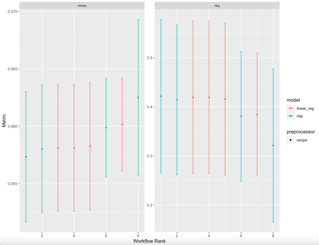
Using rmse and rsq, it is also visually clear the the basic neural network has the best results, though the tradeoff for using others is not substantial. It is up to the user to determine if a more intuitive model would be preferred; in fact, Bayesian analysis is available to determine effect size differences.
Conclusion
This tutorial scratches the surface of how tidymodels can be applied to sports data. Dozens of other models, classification problems and variable selection are other avenues any data scientist can travel to further master this package. There are several other resources I suggest reading beyond what has already been listed, but perhaps the most thorough can be found here.
Adapting Two-Way ANOVA Presentation
For my lesson on including a second grouping variable to the ANOVA experience, I came across this presentation. The background information is elegant, the data visualizations are clear and the opportunities to learn more are sprinkled throughout. The only problem with the lesson was this is an English dataset. Specifically, the dataset involves job satisfaction among education levels, and the dataset uses the terms “school”, “college” and “university” to refer to compulsory school, a two-year program to prepare for university, then undergraduate and beyond, respectively.
Because I did not want to distract my students from the statistical lesson, I wanted to use the tidyverse to rename these education levels to something more American: high school, undergraduate and postgrad:
jobsatisfaction <- jobsatisfaction %>%
  mutate(education_level = str_replace(education_level, "school",
                                       "High School")) %>%
  mutate(education_level = str_replace(education_level, "college",
                                       "Undergrad")) %>%
  mutate(education_level = str_replace(education_level, "university",
                                       "Postgrad"))
While I wanted the next step to be exploratory data analysis with boxplots, there was just one problem: R automatically alphabetizes these new education levels. It would make more intuitive sense to have Postgrad after Undergrad. To make this change, I used the factor command:
jobsatisfaction$education_level <-
  factor(jobsatisfaction$education_level,
         levels = c("High School", "Undergrad", "Postgrad"))
From there I was able to walk through the rest of the tutorial with ease. It is one I would highly recommend if you are learning/teaching any ANOVA approach.
Randomly Splitting a Class of Students Into Groups
One of the temptations I have when creating group activities in class is to lean on the location of where students are sitting to divide accordingly. Given all of the research concerning how important it is to promote diversity of thought, it would behoove everyone to randomly create pairings and groups among the class.
Originally, I used the sample command to randomly assign anything, but the split command is more effective. This line simply divides a vector into various parts. I am using a base R approach, but certainly slice in dplyr can also be utilized. In my case, I am looking to divide my class of 12:
#To create reproducible results
set.seed(123)

#Create an object called students
students <- as.data.frame(c("Joe", "Cynthia", "Lisa", "Monica", "Emily", "Aaron", "Bobby", "Zoe", "Vanessa", "Chloe", "Brandy", "Jen"))
students <- unname(students) #No headers necessary

#Randomize the students
random_students <- students[sample(nrow(students)),]

#To create pairs
split(random_students,rep(1:6,each=2))

#Or to create groups of three
split(random_students,rep(1:4,each=3))
Depending upon the number of students, simply adjust the numbers as you see fit.
Displaying Statistical Output
Recently I showed my class how to write functions for calculating both z-tests and confidence intervals for the 68% and 95% levels. Because students analyzing these concepts for the first time deserve to have output well organized, I wanted to investigate the different ways for making these functions print results as elegant as possible. The biggest tasks are to have labels for key statistics and know when to have line breaks.
As with most other things in R, there are options. One is cat(). Quotation marks are used for spacing and “\n” is for line breaks. For our z-test function, I utilized cat():
z.test = function(x,mu,popvar){
  one.tail.p <- NULL
  z.score <- round((mean(x)-mu)/(popvar/sqrt(length(x))),3)
  one.tail.p <- round(pnorm(abs(z.score),lower.tail = FALSE),3)
  cat(" z =",z.score,"\n",
      "one-tailed probability =", one.tail.p,"\n",
      "two-tailed probability =", 2*one.tail.p )}
where “x” is the sample vector, “mu” is the mean of the population and “popvar” is the variance of the population. Here, the first line is “z = ” then the z-score, then a line break, then the probability labels and their corresponding p-values. So if an IQ vector were used with a mean of 100 and an sd of 15:
z = 1.733
one-tailed probability = 0.042

two-tailed probability = 0.084
The other option is writeLines(). This command is more concise because you don’t need “\n” for line breaks. Here’s how I used it for our confidence intervals function:
confidence.intervals <- function(sample.size, sd, mean){
  standard.error <- sd/sqrt(sample.size)
  lower.bound <- round(mean - standard.error,2)
  upper.bound <- round(mean + standard.error,2)
  big.lower.bound <- round(mean - (1.96*standard.error),2)
  big.upper.bound <- round(mean + (1.96*standard.error),2)
  return(writeLines(c("68% CI:",
           lower.bound, upper.bound, "",
           "95% CI:", big.lower.bound, big.upper.bound)))
}
Here, anytime there is a comma, a new line is created. The sample output looks like this:
68% CI:

78.79
83.21


95% CI:
76.66

85.34
Not only do you now have options for statistical output, you have functions for computing z-tests and confidence intervals. Don’t say I never did anything for you.